Second Look

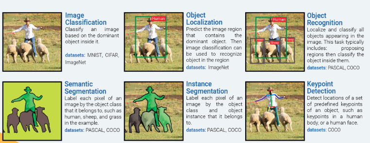
Approach: Instance Segmentation

The majority of deep learning papers have focused on the breast tumor classification problem as an “Image Classification” problem. While classifying a mammogram as “normal”, “benign”, or “malignant” is necessary, it is not sufficient to help a radiologist identify hard-to-detect tumors. Further, a mammogram image may contain multiple tumors of different types (benign/malignant). Such mammograms clearly warrant an “Instance Segmentation” approach for accurate tumor detection.
 

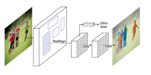
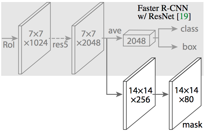
Architecture: Mask R-CNN

He et al. created Mask R-CNN by extending Faster R-CNN by adding a branch for predicting class-specific object mask for Instance Segmentation in parallel with the existing object classifier and bounding box regressor.

RoIPooling layer of Faster R-CNN is replaced by RoIAlign layer which uses bilinear interpolation to calculate a segmentation mask at a pixel by pixel level.

Data Preprocessing

1. Dataset Selection

The CBIS-DDSM dataset has four sub datasets: Mass-Training, Mass-Test, Calc-Training and Calc-Test. Mass-Training has images for 1318 tumors. Mass-Test has images for 378 tumors. Calc-Training has images for 1622 calcifications. Calc-Test has images for 326 calcifications. For this project, we used the Mass-Training and Mass-Test datasets only.

The Mass-Training dataset has images for 637 'Malignant' tumors, 577 'Benign' tumors, and 104 'Benign without callback' tumors. We combined 'Benign' and 'Benign without callback' into a single 'Benign' class which has images for 681 tumors. All of them have corresponding segmentation masks available as the ground truth.

The Mass-Test dataset has images for 147 'Malignant' tumors, 194 'Benign' tumors, and 37 'Benign without callback' tumors. We combined 'Benign' and 'Benign without callback' into a single 'Benign' class which has images for 231 tumors. All of them have corresponding segmentation masks available as the ground truth.

The mini-MIAS dataset has images for 209 'No tumor' and 121 'Tumor' cases. Since the tumor cases do not have corresponding segmentation masks available, we did not use the 121 'Tumor' cases. We randomly split the 209 'No tumor' cases into 120 for training and 89 for testing.

2. Data Augmentation

The combined CBIS-DDSM Mass-Train (1318 cases) + mini-MIAS training (120 cases) is a small dataset. We applied data augmentation to it. We applied 6 rotations (100, 200, 300, -100, -200, -300 ) and created a total of CBIS-DDSM Mass-Train (9226 cases) + mini-MIAS training (840 cases). Then we flipped all of those images horizontally and created a total of CBIS-DDSM Mass-Train (18,452 cases) + mini-MIAS training (1680 cases).

The combined CBIS-DDSM Mass-Test (378 cases) + mini- MIAS test (98 cases) is a small dataset. We applied data augmentation to it. We applied 6 rotations (100, 200, 300, -100, -200, -300 ) and created a total of CBIS-DDSM Mass-Test (2646 cases) + mini-MIAS test (686 cases). Then we flipped all of those images horizontally and created a total of CBIS- DDSM Mass-Test (5292 cases) + mini-MIAS test (1372 cases).

During mammogram acquisition, the technicians ensure that breasts are properly positioned when acquiring craniocaudal (CC) and mediolateral oblique (MLO) views. This ensures that the nipples are close to the center of the image. Hence, we chose not to apply translations to mammograms as it is highly unlikely to have a mammogram with the nipple farther away from the image center.

3. Patch Extraction

The CBIS-DDSM Mass-Train (18,452 cases) dataset has image sizes varying from 2000 x 2000 to 5000 x 5000 pixels. The mini-MIAS training (1680 cases) dataset has all images with size 1024 x 1024 pixels. The smallest tumor in CBIS-DDSM is 54 x 85 pixels. The Mask R-CNN can accept 256 x 256 images without resizing. A 2k x 2k image resized to 256 x 256 will result in 8 times reduction in width/height and 64 times reduction in area. It will be 20 times reduction in width/height and 400 times reduction in area. Small tumors will shrink so much with such reductions, that it will become impossible for the network to learn their morphology. Since, small tumors are also harder to detect for the radiologists, it is necessary that the network can detect small tumors with high accuracy.

Hence, instead of using the whole images, we extracted patches of size 256 x 256. Many images do not have widths and heights that are a multiple of 256. So we zero padded them at right and bottom to increase their widths and heights appropriately before extracting patches.

Over 3 million 256 x 256 pixel patches were extracted from the CBIS-DDSM Mass-Train (18,452 cases) images. 26,880 patches were extracted from the mini-MIAS training (1680 cases) images. Unlike the original images that had tumors, surrounding breast tissue and black background in each mammogram; a majority of the patches had only the black background, only the breast tissue without tumor or a combination of the black background with the breast tissue without tumor. About 250,000+ patches had either just tumor or tumor with surrounding breast tissue and the black background.

We kept all 250,000 patches with breast tumor and sampled 300,000 patches that had 100,000 black background, 100,000 breast tissue, and 100,000 black background with breast tissue. We used this dataset to train Mask R-CNN.

The CBIS-DDSM Mass-Test (5292 cases) dataset has image sizes varying from 2000 x 2000 to 5000 x 5000 pixels. The mini-MIAS test (1327 cases) dataset has all images with size 1024 x 1024 pixels.

846,720 256 x 256 pixel patches were extracted from the CBIS-DDSM Mass-Test (5292 cases) images. 21,952 patches were extracted from the mini-MIAS training (1372 cases) images. We used all of those patches for testing.

Network Architecture

We derived our Mask R-CNN architecture based on the Functional Pyramid Network (FPN) variant of Mask R-CNN.

Feature Pyramid Network extracts features at different scales based on their levels in the feature pyramid. The ResNet – FPN backbone provides good accuracy without sacrificing speed.

Our Mask R-CNN architecture leverages and extends the framework of Abdullah et al. at Matterport. Our Mask R-CNN model has – 63,744,170 total parameters, 63,632,682 trainable parameters, and 111,488 non-trainable parameters.

Training & Testing

We used Google Cloud Platform virtual machines for training and testing. Our virtual machine environment had the following specifications:

1. Zone: us-west1-b
2. Machine type: n1-standard-4
3. CPUs: 4 vCPUs (unknown CPU platform)
4. CPU RAM: 15 GB
5. GPU: 1 Nvidia Tesla K80 (half board)
6. GPU RAM: 12 GB
7. HDD: 1 TB persistent storage
8. OS: Ubuntu 16.04.3 LTS
9. Nvidia CUDA: CUDA 8.0.61
10. Nvidia cuDNN: cuDNN 6.0.21
11. Google Tensorflow: TensorFlow 1.3.0
12. Keras: Keras 2.0.8
13. OpenCV: OpenCV 3.3.0
14. Jupyter Notebook: Jupyter Notebook 5.1.0

On Google Cloud Platform, Tesla P100 GPUs cost 3 times Tesla K80 GPUs. However, while using Tesla P100 GPUs, there was only a 30-40% performance increase over Tesla K89 GPUs. Hence, we used K80 GPUs for the bulk of our training and testing activities as they had a better performance/price ratio. We used Mask-RCNN pretrained on the COCO dataset.

We observed that Mask-RCNN requires a large amount of memory and hence we could only train 2 images in a batch per GPU in the available environment reliably without experiencing memory errors. This small batch size was equivalent to stochastic training instead of a mini-batch training. To maintain the network stability we were forced to use a lower learning rate of 0.002 which we had to reduce in later epochs to 0.0002.

The video below shows the Second Look user interface:

 

To see a demo of the solution, please follow these steps:

1. Build and launch the repository by clicking this link.
2. Navigate to the "inference" folder.
3. Open "ROIBreastTumorsDataset-Patches-Demo.ipynb"
4. Execute code from start to the "Ground Truth" section once.
5. The "Ground Truth" and "Prediction" sections can be executed multiple times - every time the code will choose a random image, and show the ground truth and prediction.

When we split images into patches, we observed that many tumors got split unevenly into two or more patches where one or two patches contained the majority of the tumor portions and the remaining patches contained very small tumor portions. Those very small tumor portions did not seem to have any characteristic features of tumors (e.g. microcalcifications, mass morphology etc.) for Mask R-CNN to identify them as parts of the tumors, just based on the small portion in a single patch alone. We expected Mask R-CNN to fail to identify those small portions of tumors and observed the same.

Hence, we calculated prediction accuracy at both the patch level and image level. Let's look at an example. An image containing a tumor is split into 4 patches, where one patch contains the majority of the tumor, another part contains a small portion of the tumor and the remaining two patches contain no tumor. Mask R-CNN identifies the patch with the majority of the tumor as “tumor”, the patch with the small portion of the tumor as “no tumor” and the two patches with “no tumor” as “no tumor”. The patch level accuracy = 3 correct predictions out of 4 predictions = 0.75. When we consider the whole image, one patch that contained the majority of the tumor was correctly identified by Mask RCNN as “tumor”. Hence the image level accuracy = 1 correct prediction out of 1 total predictions = 1.0.

Using the methodology described above, we calculated prediction accuracy and the area under the receiver operating characteristic curve for patches and images.

No.	Type	Accuracy	AUC
1	Patches	0.83	0.73
2	Images	1	0.93